Steps 1-6
- Load the R packages we will use.
- Read the data in the files,
drug_cos.csv,health_cos.csvin to R and assign to the variablesdrug_cosandhealth_cos, respectively
drug_cos  <- read_csv("https://estanny.com/static/week6/drug_cos.csv")
health_cos  <- read_csv("https://estanny.com/static/week6/health_cos.csv")
- Use glimpse to get a glimpse of the data
drug_cos %>% glimpse()
Rows: 104
Columns: 9
$ ticker       <chr> "ZTS", "ZTS", "ZTS", "ZTS", "ZTS", "ZTS", "ZTS…
$ name         <chr> "Zoetis Inc", "Zoetis Inc", "Zoetis Inc", "Zoe…
$ location     <chr> "New Jersey; U.S.A", "New Jersey; U.S.A", "New…
$ ebitdamargin <dbl> 0.149, 0.217, 0.222, 0.238, 0.182, 0.335, 0.36…
$ grossmargin  <dbl> 0.610, 0.640, 0.634, 0.641, 0.635, 0.659, 0.66…
$ netmargin    <dbl> 0.058, 0.101, 0.111, 0.122, 0.071, 0.168, 0.16…
$ ros          <dbl> 0.101, 0.171, 0.176, 0.195, 0.140, 0.286, 0.32…
$ roe          <dbl> 0.069, 0.113, 0.612, 0.465, 0.285, 0.587, 0.48…
$ year         <dbl> 2011, 2012, 2013, 2014, 2015, 2016, 2017, 2018…
health_cos %>% glimpse()
Rows: 464
Columns: 11
$ ticker      <chr> "ZTS", "ZTS", "ZTS", "ZTS", "ZTS", "ZTS", "ZTS"…
$ name        <chr> "Zoetis Inc", "Zoetis Inc", "Zoetis Inc", "Zoet…
$ revenue     <dbl> 4233000000, 4336000000, 4561000000, 4785000000,…
$ gp          <dbl> 2581000000, 2773000000, 2892000000, 3068000000,…
$ rnd         <dbl> 427000000, 409000000, 399000000, 396000000, 364…
$ netincome   <dbl> 245000000, 436000000, 504000000, 583000000, 339…
$ assets      <dbl> 5711000000, 6262000000, 6558000000, 6588000000,…
$ liabilities <dbl> 1975000000, 2221000000, 5596000000, 5251000000,…
$ marketcap   <dbl> NA, NA, 16345223371, 21572007994, 23860348635, …
$ year        <dbl> 2011, 2012, 2013, 2014, 2015, 2016, 2017, 2018,…
$ industry <chr> "Drug Manufacturers - Specialty & Generic", "Dr…- Which variables are the same in both data sets
names_drug  <- drug_cos  %>%  names()
names_health  <- health_cos  %>%  names()
intersect(names_drug, names_health)
[1] "ticker" "name" "year" - Select subset of variables to work with
For
drug_cosselect (in this order):ticker,year,grossmarginExtract observations for 2018
Assign output to
drug_subset
For
health_cosselect (in this order):ticker,year,revenue,gp,industryExtract observations for 2018
Assign output to
health_subset
- Keep all the rows and columns
drug_subsetjoin with columns inhealth_subset
drug_subset %>% left_join(health_subset)
# A tibble: 13 x 6
   ticker  year grossmargin   revenue        gp industry
   <chr>  <dbl>       <dbl>     <dbl>     <dbl> <chr>
 1 ZTS     2018       0.672   5.82e 9   3.91e 9 Drug Manufacturers - …
 2 PRGO    2018       0.387   4.73e 9   1.83e 9 Drug Manufacturers - …
 3 PFE     2018       0.79    5.36e10   4.24e10 Drug Manufacturers - …
 4 MYL     2018       0.35    1.14e10   4.00e 9 Drug Manufacturers - …
 5 MRK     2018       0.681   4.23e10   2.88e10 Drug Manufacturers - …
 6 LLY     2018       0.738   2.46e10   1.81e10 Drug Manufacturers - …
 7 JNJ     2018       0.668   8.16e10   5.45e10 Drug Manufacturers - …
 8 GILD    2018       0.781   2.21e10   1.73e10 Drug Manufacturers - …
 9 BMY     2018       0.71    2.26e10   1.60e10 Drug Manufacturers - …
10 BIIB    2018       0.865   1.35e10   1.16e10 Drug Manufacturers - …
11 AMGN    2018       0.827   2.37e10   1.96e10 Drug Manufacturers - …
12 AGN     2018       0.861   1.58e10   1.36e10 Drug Manufacturers - …
13 ABBV    2018       0.764   3.28e10   2.50e10 Drug Manufacturers - …
Question: join_ticker
Start with
drug_cosExtract observations for the ticker MYL from
drug_cosAssign output to the variable
drug_cos_subset
drug_cos_subset  <- drug_cos  %>%
  filter(ticker == "MYL")
- Display drug_cos_subset
drug_cos_subset
# A tibble: 8 x 9
  ticker name  location ebitdamargin grossmargin netmargin   ros   roe
  <chr>  <chr> <chr>           <dbl>       <dbl>     <dbl> <dbl> <dbl>
1 MYL    Myla… United …        0.245       0.418     0.088 0.161 0.146
2 MYL    Myla… United …        0.244       0.428     0.094 0.163 0.184
3 MYL    Myla… United …        0.228       0.44      0.09  0.153 0.209
4 MYL    Myla… United …        0.242       0.457     0.12  0.169 0.283
5 MYL    Myla… United …        0.243       0.447     0.09  0.133 0.089
6 MYL    Myla… United …        0.19        0.424     0.043 0.052 0.044
7 MYL    Myla… United …        0.272       0.402     0.058 0.121 0.054
8 MYL    Myla… United …        0.258       0.35      0.031 0.074 0.028
# … with 1 more variable: year <dbl>
Use left_join to combine the rows and columns of
drug_cos_subsetwith the columns ofhealth_cosAssign the output to
combo_df
combo_df  <- drug_cos_subset  %>%
  left_join(health_cos)
- Display
combo_df
combo_df
# A tibble: 8 x 17
  ticker name  location ebitdamargin grossmargin netmargin   ros   roe
  <chr>  <chr> <chr>           <dbl>       <dbl>     <dbl> <dbl> <dbl>
1 MYL    Myla… United …        0.245       0.418     0.088 0.161 0.146
2 MYL    Myla… United …        0.244       0.428     0.094 0.163 0.184
3 MYL    Myla… United …        0.228       0.44      0.09  0.153 0.209
4 MYL    Myla… United …        0.242       0.457     0.12  0.169 0.283
5 MYL    Myla… United …        0.243       0.447     0.09  0.133 0.089
6 MYL    Myla… United …        0.19        0.424     0.043 0.052 0.044
7 MYL    Myla… United …        0.272       0.402     0.058 0.121 0.054
8 MYL    Myla… United …        0.258       0.35      0.031 0.074 0.028
# … with 9 more variables: year <dbl>, revenue <dbl>, gp <dbl>,
#   rnd <dbl>, netincome <dbl>, assets <dbl>, liabilities <dbl>,
# marketcap <dbl>, industry <chr>- Note: the variables
ticker,name,locationandindustryare the same for all the observations
- Assign the company name to
co_name
co_name  <- combo_df  %>%
  distinct(name) %>%
  pull()
- Assign the company location to
co_location
co_location  <- combo_df  %>%
  distinct(name)  %>%
  pull()
- Assign the industry to co_industry group
co_industry  <- combo_df  %>%
  distinct(name)  %>%
  pull()
Put the r inline commands used in the blanks below. When you knit the document the results of the commands will be displayed in your text.
The company co_name is located in co_location and is a member of the co_industry industry group.
Start with
combo_dfSelect variables (in this order):
year,grossmargin,netmargin,revenue,gp,netincomeAssign the output to
combo_df_subset
combo_df_subset  <- combo_df  %>%
  select(year, grossmargin, netmargin,
  revenue, gp, netincome)
- Display combo_df_subset
combo_df_subset
# A tibble: 8 x 6
   year grossmargin netmargin     revenue         gp netincome
  <dbl>       <dbl>     <dbl>       <dbl>      <dbl>     <dbl>
1  2011       0.418     0.088  6129825000 2563364000 536810000
2  2012       0.428     0.094  6796100000 2908300000 640900000
3  2013       0.44      0.09   6909100000 3040300000 623700000
4  2014       0.457     0.12   7719600000 3528000000 929400000
5  2015       0.447     0.09   9429300000 4216100000 847600000
6  2016       0.424     0.043 11076900000 4697000000 480000000
7  2017       0.402     0.058 11907700000 4783100000 696000000
8 2018 0.35 0.031 11433900000 4001600000 352500000- Create the variable
grossmargin_checkto compare with the variablegrossmargin. They should be equal.- `
grossmargin_check=gp/revenue
- `
- Create the variable
close_enoughto check that the absolute value of the difference betweengrossmargin_checkandgrossmarginis less than 0.001
combo_df_subset  %>%
  mutate(grossmargin_check = gp / revenue,
  close_enough = abs(grossmargin_check - grossmargin) < 0.001)
# A tibble: 8 x 8
   year grossmargin netmargin revenue     gp netincome
  <dbl>       <dbl>     <dbl>   <dbl>  <dbl>     <dbl>
1  2011       0.418     0.088 6.13e 9 2.56e9 536810000
2  2012       0.428     0.094 6.80e 9 2.91e9 640900000
3  2013       0.44      0.09  6.91e 9 3.04e9 623700000
4  2014       0.457     0.12  7.72e 9 3.53e9 929400000
5  2015       0.447     0.09  9.43e 9 4.22e9 847600000
6  2016       0.424     0.043 1.11e10 4.70e9 480000000
7  2017       0.402     0.058 1.19e10 4.78e9 696000000
8  2018       0.35      0.031 1.14e10 4.00e9 352500000
# … with 2 more variables: grossmargin_check <dbl>,
#   close_enough <lgl>
Create the variable
netmargin_checkto compare with the variablenetmargin. They should be equal.Create the variable
close_enoughto check that the absolute value of the difference betweennetmargin_checkandnetmarginis less than 0.001
combo_df_subset  %>%
  mutate(netmargin_check = gp / revenue,
  close_enough = abs(netmargin_check - netmargin) < 0.001)
# A tibble: 8 x 8
   year grossmargin netmargin revenue     gp netincome netmargin_check
  <dbl>       <dbl>     <dbl>   <dbl>  <dbl>     <dbl>           <dbl>
1  2011       0.418     0.088 6.13e 9 2.56e9 536810000           0.418
2  2012       0.428     0.094 6.80e 9 2.91e9 640900000           0.428
3  2013       0.44      0.09  6.91e 9 3.04e9 623700000           0.440
4  2014       0.457     0.12  7.72e 9 3.53e9 929400000           0.457
5  2015       0.447     0.09  9.43e 9 4.22e9 847600000           0.447
6  2016       0.424     0.043 1.11e10 4.70e9 480000000           0.424
7  2017       0.402     0.058 1.19e10 4.78e9 696000000           0.402
8  2018       0.35      0.031 1.14e10 4.00e9 352500000           0.350
# … with 1 more variable: close_enough <lgl>
Question: summarize_industry
Fill in the blanks
Put the command you use in the Rchunks in the Rmd file for this quiz
Use the health_cos data
For each industry calculate
- mean_grossmargin_percent = mean(gp / revenue) * 100
- median_grossmargin_percent = median(gp / revenue) * 100
- min_grossmargin_percent = min(gp / revenue) * 100
- max_grossmargin_percent = max(gp / revenue) * 100
health_cos  %>%
  group_by(industry)  %>%
  summarize(mean_grossmargin_percent = mean(gp / revenue) * 100
            ,
            median_grossmargin_percent = median(gp / revenue) * 100,
            min_grossmargin_percent = min(gp / revenue) * 100,
            max_grossmargin_percent = max(gp / revenue) * 100
  )
# A tibble: 9 x 5
  industry mean_grossmargi… median_grossmar… min_grossmargin…
* <chr>               <dbl>            <dbl>            <dbl>
1 Biotech…             92.5            92.7             81.7
2 Diagnos…             50.5            52.7             28.0
3 Drug Ma…             75.4            76.4             36.8
4 Drug Ma…             47.9            42.6             34.3
5 Healthc…             20.5            19.6             10.0
6 Medical…             55.9            37.4             28.1
7 Medical…             70.8            72.0             53.2
8 Medical…             10.4             5.38             2.49
9 Medical…             53.9            52.8             40.5
# … with 1 more variable: max_grossmargin_percent <dbl>- mean_grossmargin_percent for the industry Medical Devices is 70.8%
- median_grossmargin_percent for the industry Medical Devices is 72.0%
- min_grossmargin_percent for the industry Medical Devices is 53.2%
- max_grossmargin_percent for the industry Medical Devices is 84.7%
Question: inline_ticker
Fill in the blanks
Use the
health_cos dataExtract observations for the ticker BMY from `
health_cosand assign to the variablehealth_cos_subset
health_cos_subset  <- health_cos  %>%
  filter(ticker == "BMY")
- Display
health_cos_subset
health_cos_subset
# A tibble: 8 x 11
  ticker name  revenue      gp    rnd netincome  assets liabilities
  <chr>  <chr>   <dbl>   <dbl>  <dbl>     <dbl>   <dbl>       <dbl>
1 BMY    Bris… 2.12e10 1.56e10 3.84e9    3.71e9 3.30e10 17103000000
2 BMY    Bris… 1.76e10 1.30e10 3.90e9    1.96e9 3.59e10 22259000000
3 BMY    Bris… 1.64e10 1.18e10 3.73e9    2.56e9 3.86e10 23356000000
4 BMY    Bris… 1.59e10 1.19e10 4.53e9    2.00e9 3.37e10 18766000000
5 BMY    Bris… 1.66e10 1.27e10 5.92e9    1.56e9 3.17e10 17324000000
6 BMY    Bris… 1.94e10 1.45e10 5.01e9    4.46e9 3.37e10 17360000000
7 BMY    Bris… 2.08e10 1.47e10 6.48e9    1.01e9 3.36e10 21704000000
8 BMY    Bris… 2.26e10 1.60e10 6.34e9    4.92e9 3.50e10 20859000000
# … with 3 more variables: marketcap <dbl>, year <dbl>,
#   industry <chr>
In the console, type
?distinct. Go to the help pane to see whatdistinctdoesIn the console, type
?pull. Go to the help pane to see whatpulldoes
run the code below
health_cos_subset  %>%
  distinct(name) %>%
  pull(name)
[1] "Bristol Myers Squibb Co"- Assign the output to co_name?
co_name <- health_cos_subset  %>%
  distinct(name) %>%
  pull(name)
You can take output from your code and include it in your text.
- The name of the company with ticker BMY is Bristol Myers Squibb Co
In following chuck
- Assign the company’s industry group to the variable
co_industry
co_industry  <- health_cos_subset  %>%
  distinct(industry) %>%
  pull()
This is outside the R chunk. Put the r inline commands used in the blanks below. When you knit the document the results of the commands will be displayed in your text.
The company Bristol Myers Squibb Co is a member of the Drug Manufacturers - General group.
Steps 7-11
- Prepare the data for the plots
- start with health_cos THEN
- group_by industry THEN
- calculate the median research and development expenditure by industry
- assign the output to
df
- Use glimpse to glimpse the data for the plots
df %>% glimpse()
Rows: 9
Columns: 2
$ industry    <chr> "Biotechnology", "Diagnostics & Research", "Dru…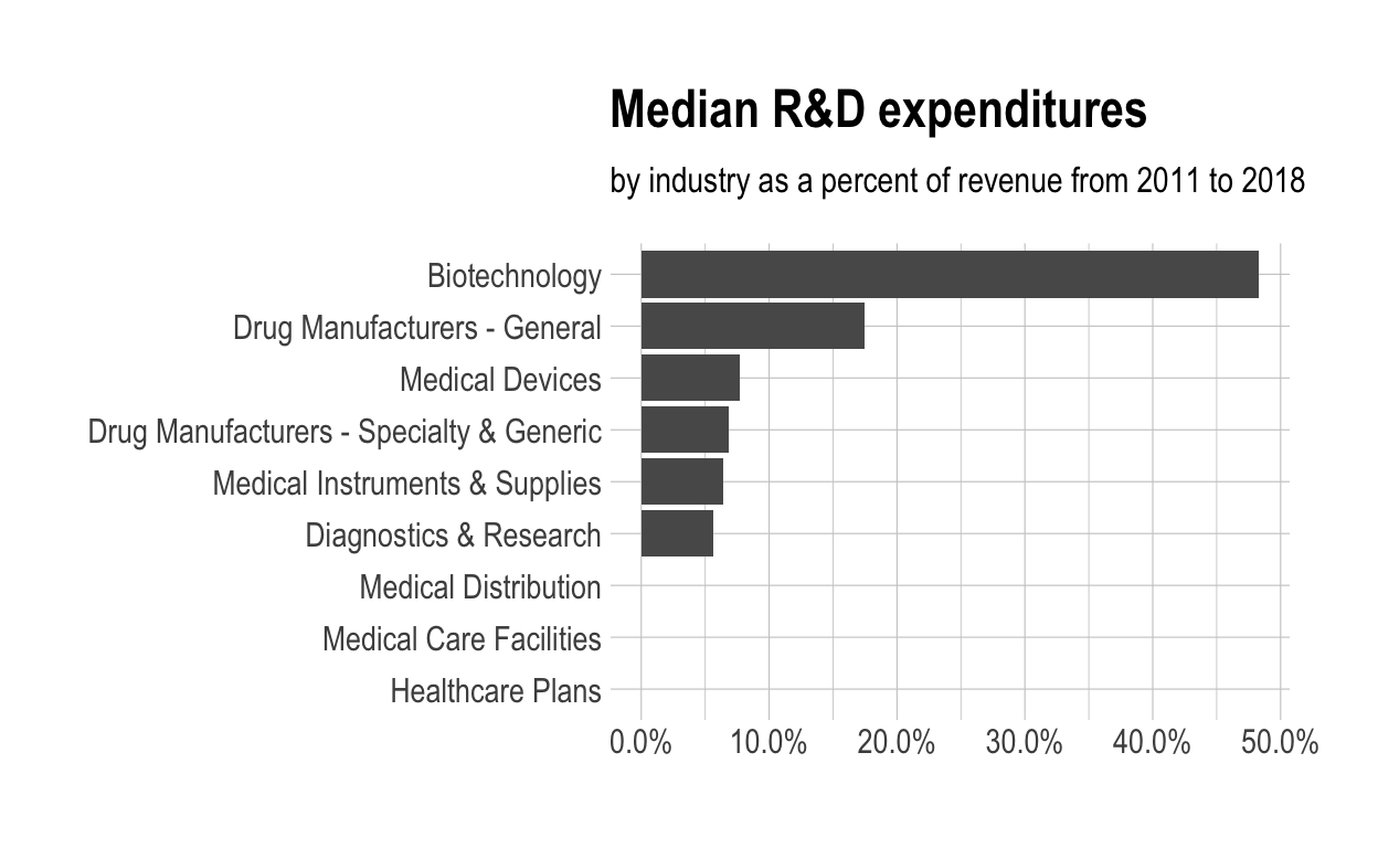
$ med_rnd_rev <dbl> 0.48317287, 0.05620271, 0.17451442, 0.06851879,…- Create a static bar chart
- use ggplot to initialize the chart
- data is df
- the variable industry is mapped to the x-axis reorder it based the value of med_rnd_rev
- the variable med_rnd_rev is mapped to the y-axis
- add a bar chart using geom_col
- use scale_y_continuous to label the y-axis with percent
- use coord_flip() to flip the coordinates
- use labs to add title, subtitle and remove x and y-axes
- use theme_ipsum() from the hrbrthemes package to improve the theme
ggplot(data = df,
       mapping = aes(
         x = reorder(industry, med_rnd_rev ),
         y = med_rnd_rev
         )) +
  geom_col() +
  scale_y_continuous(labels = scales::percent) +
  coord_flip() +
  labs(
    title = "Median R&D expenditures",
    subtitle = "by industry as a percent of revenue from 2011 to 2018",
    x = NULL, y = NULL) +
  theme_ipsum()
- Save the last plot to preview.png and add to the yaml chunk at the top
ggsave(filename = "preview.png",
       path = here::here("_posts", "2021-03-01-joining-data"))
- Create an interactive bar chart using the package echarts4r
- start with the data
df - use
arrangeto reordermed_rnd_rev - use
e_chartsto initialize a chart the variableindustryis mapped to the x-axis - add a bar chart using
e_barwith the values ofmed_rnd_rev - use
e_flip_coords()to flip the coordinates - use
e_titleto add the title and the subtitle - use
e_legendto remove the legends - use
e_x_axisto change format of labels on x-axis to percent - use
e_y_axisto remove labels on y-axis- - use
e_themeto change the theme. Find more themes here
df  %>%
  arrange(med_rnd_rev)  %>%
  e_charts(
    x = industry
    )  %>%
  e_bar(
    serie = med_rnd_rev,
    name = "median"
    )  %>%
  e_flip_coords()  %>%
  e_tooltip()  %>%
  e_title(
    text = "Median industry R&D expenditures",
    subtext = "by industry as a percent of revenue from 2011 to 2018",
    left = "center") %>%
  e_legend(FALSE) %>%
  e_x_axis(
    formatter = e_axis_formatter("percent", digits = 0)
    )  %>%
  e_y_axis(
    show = FALSE
  )  %>%
  e_theme("infographic")